A More Accurate and Encouraging Assessment of Basic Controls of Life Expectancy in the Lower 48 American States

Reading this particular post is likely to be slow, difficult slogging for a lot of people, however.

Introduction

The health-related sciences are largely binary in their measurements and pronouncements when it comes to assessing the relative effects of various actions and habits on human lifespan.  There is little to no information as to how various positive and negative actions and habits come together to increase or decrease lifespan.  Mostly the scientific literature and medical advice available to homo sapiens has the nigh on useless nature of being a disorganized and disconnected series of one-dimensional maps; i.e., such and such is bad for you, while such and such is good for you – and on and on.  Makes it hard to map out a course of behavior.

The writer’s purpose in carrying out the Cobb-Douglas linear regression of certain apparent controls of human longevity in the Lower 48 States – as reported in the previous post - was to inquire which, if any, of those controls might be most critical in establishing relatively greater longevity in the people living in the nation. In other words, the idea was conduct some simple mathematical exploration in order to draft a rough, two-dimensional map of the apparent causes of US human longevity (and associated good health).

The last post explained, however, that the accuracy of the log-linear form of the Cobb-Douglas production is limited by its mathematical rigidity when conducting linear regression of controlling variables (inputs) against an output (e.g., COVID19 mortality rates or state resident life expectancy). The Cobb-Douglas equation, that probably the most commonly used in linear regressions of observational data by scientists of all stripes, does not allow the coefficients (i.e., the output elasticities) of the controlling (independent) variables estimated by the linear regression procedure to vary with change in the size of the output (the dependent variable), or with change in the values of any of the controlling variables.  This is a very severe deficiency when seeking to accurately describe a world that is actually made up of interdependent, cooperating, and/or conflicting entities and processes.

The log-linear¹ translog production function, in contrast to the log-linear Cobb-Douglas production function model, is much more flexible and permits statistically-based detection of controlling variable coefficients that more realistically change with the ‘matrix effects’ of different natural input-output system states.  Accordingly, provided the controlling variables are chosen appropriately and the data denoting different cases of the controlling variables are sufficiently accurate, linear regression of a translog model of a production system based on a given set of inputs will be much more predictive and theoretically accurate than linear regression of a Cobb-Douglas model of the same system. In other words, linear regression using the translog model reveals much more potentially actionable information than the simpler Cobbs-Douglas model because it comes considerably closer to accurately representing nature.

Table I and Table II demonstrate the measured statistical differences between the two models.  Levels of significance for the translog model estimates of the input variable coefficients are generally much higher than seen in the Cobb Douglas model, and the coefficient of determination (the r-squared value) indicates the translog model predicts as much as 97% of the state-to-state variation in life expectancy.  In contrast, the Cobb-Douglas model only predicts about 91% of expected resident lifespan in any given state. Linear regression of the translog model also realistically tests for second power (variable squared: v1*v1)² and complementary relationships (e.g., v1*v2) among the controlling variables. See Figure 1 below to see the mathematical form of the translog linear regression model.

The previous post defines the variables referenced in Table I and Table II, as does this footnote.³

Table I.  Cobb-Douglas model of life expectancy (LE) controls in the Lower 48 States.  The coefficients shown are already equal to the output elasticities of the variables.

Table II. The translog model of the life expectancy (LE) in the Lower 48 States.  The coefficients shown are not already equivalent to the output elasticities of the controlling variables shown.  The second equation shown in Figure 1 below needs to be used to convert the Table II coefficients to output elasticities for each of the controlling variables of the translog model of state average life expectancy.

Figure 1. Translog linear equation and input variable output elasticity formulas.

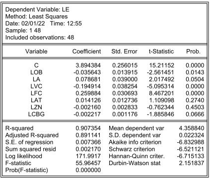
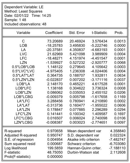
The calculation of each of the output elasticities of the individual controlling variables (LOB, LA, LVC, LFC, LZN, LAT, and LCBG) extremely surprisingly and encouragingly indicates that a 10% overall increase in certain of these controlling variables, and an overall 10% decrease in select others, could result in statewide average life expectancy increases in slight excess of 55%.

This very improbable-sounding effect would ostensibly take the US national current average life expectancy (both sexes) of about 78 years up to about 121 years; i.e., very close to the 122 ½ year old age of death of the currently longest-ever living person on verified record, Jeanne Calment.

Figure 2.  From https://en.wikipedia.org/wiki/Jiroemon_Kimura.  Photo of Jiroemon Kimura on his 115th birthday – about a year before his death at the age of 116.  Kimura is, to date, the longest living modern age human male.  Kimura was not obese and physically worked on the family farm until he reached the age of 90. 

 If these modeling results are even moderately accurate, this raises the distinct possibility that life expectancy-limiting personal characteristics such as sloth and gluttony might actually be human behaviors favored by natural selection -- in a short run world of limited resources, that is.  Better, perhaps, says Mother Nature, that the world population be partially kept in check by delimited longevity caused by a lot of people who act in ways that aren’t good for them and their physical bodies at all.

The next section of this posting provides the respective estimated life expectancy output elasticities for the seven (7) controlling variables used in the translog linear regression of Lower 48 State life expectancies, identifies the most important controlling variables leading to increased state population life expectancy, and illustrates how those elasticities apparently affecting long run life expectancy vary quite markedly among the 48 Lower States.⁴

Comparative Strengths of the Basic Controls of Life Expectancy in the Lower 48

Keep in mind that the modeling results provided here are provisional estimates that need to be tested with larger and more specific sample sets (and/or with personal or academic experimentation), and are directly related to the average life expectancy of state populations as a whole, and not to the longevity of individual humans. The directions of influence on individual life expectancy should be the same, however, as they are with population life expectancy.

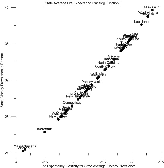
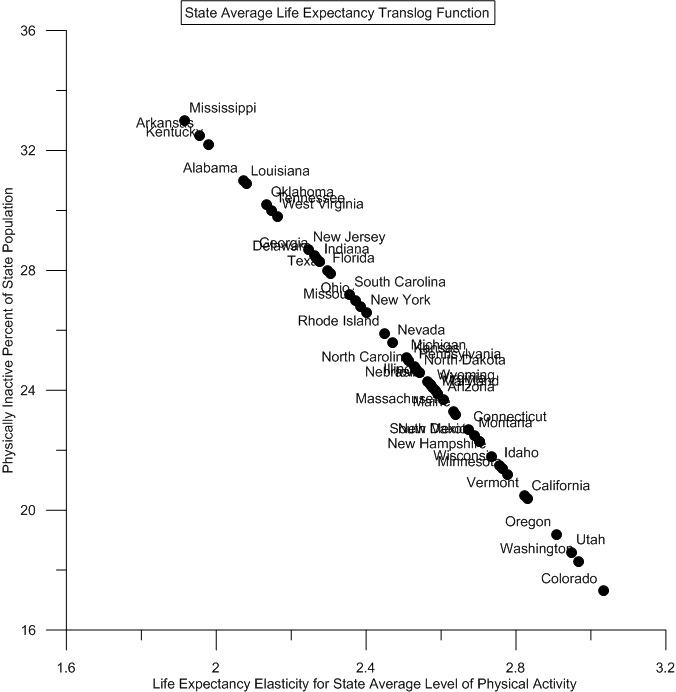
Table III shows the computed average state output elasticities for the seven controlling variables used in the translog modeling of average life expectancy of the 48 different lower 48 US states.  By far, the most critical controlling variables in determining average state life expectancy are obesity(↓) and exercise(↑).  According to the linear regression modeling results, increasing overall state population physical activity level by 10% would net the population of the average US state about a 25% increase in life expectancy.  On the other hand, decreasing overall state population obesity rates by 10% would similarly net the average state about a 26% increase in the life expectancy of its residents.

The Matters of Vegetables, Obesity, and Exercise

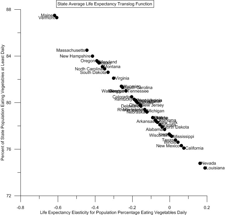
It was a wholly unanticipated, counterintuitive result of both the Cobb-Douglas and translog linear regression modeling of the state life expectancy data to find that vegetable consumption exerts, on the average, a negative effect on the life expectancy of US citizens.  Noting, however, that the two vegetables most consumed in the US are the potato and the tomato, the negative effect of US vegetable eating becomes more understandable.  Both of these most popular vegetables belong to the nightshade family (as do peppers, eggplant, and tobacco) and contain anomalously high concentrations of dietary poisons (phytotoxins) not denatured by normal cooking methods.⁵ Perhaps minimizing consumption of these particular vegetables most of the time is therefore warranted for the purpose of human life extension.⁶

Regarding obesity:  there do appear to be two limits to the obesity factor in human health and longevity.  Disregarding the root distortions in the body mass index (BMI) curves caused by variations in the amount of muscle mass hanging on the typically denser skeletons of those who are particularly physically fit,⁷ there is such a thing as being too thin for good health, and too fat for good health.  See Figure 3 (once again).

Figure 3.  Body Mass Index curves showing that there is a wide range of body fat load that is conducive to low mortality.  It is possible to be too fat or too skinny.  From https://www.researchgate.net/publication/263862703_Association_of_Body_Mass_Index_with_All-Cause_and_Cardiovascular_Disease_Mortality_in_the_Elderly

The question of how much and what kind of exercise is conducive to long term good health and longevity has been pretty thoroughly examined by academic and medical researchers.  A very short summary of the overall research findings can be found here. A notable quote from this very short article:

A retrospective study in JAMA attempts to answer this question. The study explores the association between long-term mortality and various levels of cardiorespiratory fitness (CRF). CRF is a measure of how well your heart and lungs pump blood and oxygen throughout the body during prolonged bouts of exercise. The more fit you are, the higher your level of CRF. Regular exercise, and vigorous exercise, can both boost CRF.

The researchers looked at over 122,000 patients at a large academic medical center who underwent exercise testing on a treadmill, an objective measure of CRF. While the average age was 53, participants ranged in age from 18 to over 80. Similar to findings of previous studies, being fit was associated with living longer. This held true at any age. The researchers also saw a relationship between CRF and survival rates: the higher the level of fitness, the higher the survival rate. This was especially notable in older people and people with high blood pressure. And the survival benefit continued to climb with no upper limit. [Emphasis added.]

Finally:  The State to State Variation in Life Expectancy-Controlling Output Elasticities

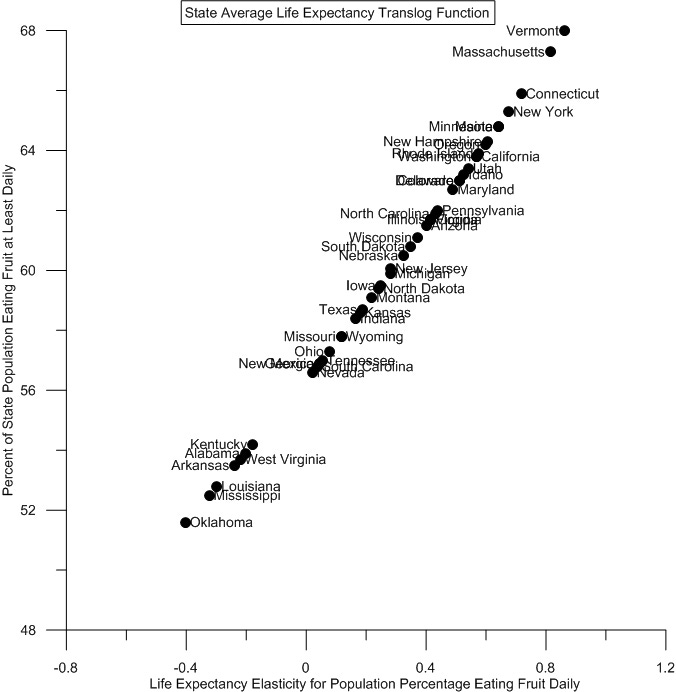
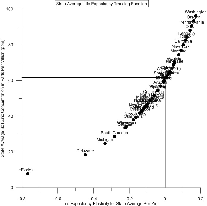
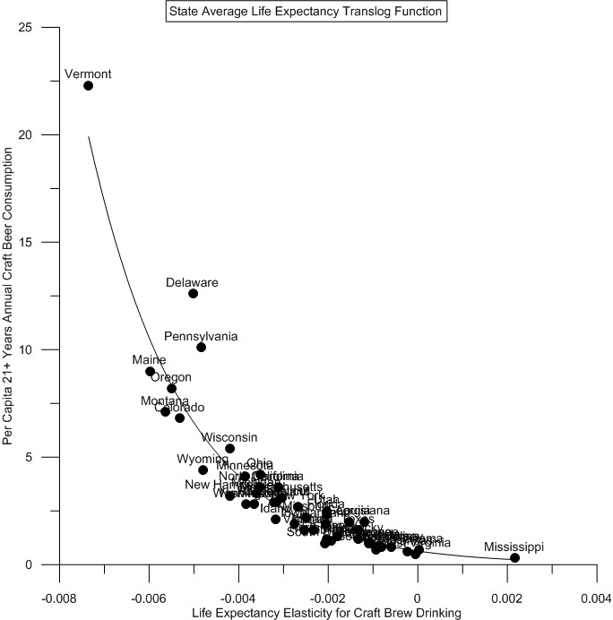
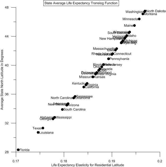
The output elasticities in Table III above are average elasticities of all 48 Lower States.  Recall, however, that the translog model allows for some variation in output elasticities depending on sample case environment.  The following series of seven scatter plots chart the controlling variable elasticities for each of the 48 states.  The exhibited output elasticity variations mean that in some states the variables ostensibly controlling the life expectancy of its citizens can – compared to all other states -- have more or less effect on the life expectancy of its citizens.

Figure 4.  State to state variations in the negative effect of obesity on state resident life expectancies.  The negative effects are relatively small for obesity increases in more obese populations like those residing in Mississippi, West Virginia, Alabama, and Louisiana – as the damage has already been done.  Decrease in life expectancy with increase in body fat in much leaner populations like those of Colorado and Massachusetts is much stronger, however.

Figure 5. State to state variations in the positive effect of exercise frequency on state resident life expectancies.  Generally speaking, this graph indicates that more of the positive effects of exercise accrue to those state populations that exhibit relatively little obesity.

Figure 6.  State to state variations in the positive and negative effects of vegetable consumption on state resident life expectancies.  Offhand and generally speaking, it is suspected that the more northern, cooler climate state populations consume more potatoes than do those people in more southern states like New Mexico, California, Nevada, and Louisiana. Potatoes in the US are mostly grown commercially and in home gardens in the cooler, more northern states.

Figure 7.  State to state variations in the positive and negative effects of fruit consumption on state resident life expectancies. It appears that the life expectancy of the more frequently obese residents of the more southern states is reduced by fruit consumption and associated fructose ingestion.  Residents of all other, more northern states evidently enjoy increased life expectancy from eating fruits.

Figure 8.  State to state variations in the positive and negative effects of soil zinc concentration on state resident life expectancies. Note that Florida, for example, has very low zinc in its soils.  This low concentration evidently reduces the state life expectancy.  Washington State soils, on the other hand, are quite rich in zinc and clearly augment the life expectancy of that state’s residents.

Figure 9.  State to state variations in the positive and negative effects of craft brew drinking on state resident life expectancies.  There is little to no positive or negative effect on life expectancy from craft brew drinking. However, remember that previously posted Cobb-Douglas modeling on COVID19 mortality rates indicated craft brew consumption decreased COVID19 mortality a bit more than did governmental lockdown measures.

Figure 10.  State to state variations in the positive effects of residential latitude on state resident life expectancies:  the further north a population lives, the greater the positive effect of latitude.  Recall this effect is hypothesized to derive from greater flu season pineal gland melatonin generation consequent of the longer duration flu season nights of the more northern states.

1. By taking an equation like c= a*b and logging the variables, the non-linear equation c= a*b becomes the linear equation log(c) = log(a)+log(b). Linear regression calculations can only work on linear equations, not on nonlinear equations like c=a*b. ‘Logging’ an equation containing variables multiplied together is therefore a clever mathematical sleight-of-hand that allows data analysis like that discussed here to be conducted.

2. What the ‘second power’ (v^2) variables of the translog model do is test and indicate whether increasing values of a given input accelerate or decelerate changes in the variable’s effect on an output like life expectancy or COVID19 mortality rate.

3. Ln = natural log; LOB (ln percent obesity prevalence); LA (ln percent of population engaging in regular exercise); LVC (ln percent of population eating at least one serving of vegetables each day); LFC (ln percent of population eating at least one serving of fruit each day); LZN (ln parts per million average state soil zinc content); LAT (ln degree average state residential latitude); and LCBG (ln number of state breweries times gallons per capita adult population consumption).

4. Remember that the translog linear regression model can ‘pick up’ and estimate the variations in output elasticities that occur from case to case – i.e., from state to state.  There are significant and telling variations among the states.

5. https://www.westonaprice.org/health-topics/food-features/nightshades/ The especially high temperatures of frying and open flame roasting reportedly can destroy nightshade vegetable toxins.  French fries and potato chips (and grilled peppers) therefore may be less damaging to human health and longevity than baked or boiled potatoes.

6. The chemical compounds found in nightshade vegetables may have material medicinal value during pandemics like COVID19, however.  See the previous post (showed a regular vegetable eating habit reduced COVID19 mortality, https://www.frontiersin.org/10.3389/conf.fphar.2010.60.00177/event_abstract, and  https://clinicaltrials.gov/ct2/show/NCT04583410. 

7. Body builders, for example, with less than 10% body fat can register as being obese using the BMI method of determining obesity. The just-retired, clearly non-obese quarterback, Tom Brady, for another example, has a BMI of a little over 29 so is supposedly overweight.  See https://www.nhlbi.nih.gov/health/educational/lose_wt/BMI/bmicalc.htm.